Tutorial 2 — Joint NMF + autoencoder

This notebook trains the joint model end-to-end and uses the resulting 2-D embedding for visualization. Useful when the downstream task is plotting / clustering rather than interpreting the W/H factors directly.

We keep the run short (10 epochs) so the notebook executes in under a minute on CPU. Production runs typically use 100+ epochs and a CUDA device.

import numpy as np
import matplotlib.pyplot as plt
import torch
torch.manual_seed(0)
np.random.seed(0)

from sparse_nmf import train_joint_model
from sparse_nmf.data import generate_synthetic_sparse

X = generate_synthetic_sparse(
    n_samples=600, n_features=800, n_components=8,
    density=0.05, seed=0,
)
print(f'shape={X.shape}  nnz={X.nnz:,}')

shape=(600, 800)  nnz=24,001

Train

nmf_components is the dimensionality of the NMF stage’s output (the autoencoder’s input). latent_dim is the bottleneck size — pick 2 for visualization, 64-256 for downstream retrieval.

z, model = train_joint_model(
    X,
    n_samples=X.shape[0],
    n_features=X.shape[1],
    nmf_components=32,
    latent_dim=2,
    device='cpu',
    n_epochs=10,
    batch_size=128,
    verbose=False,
)
z = np.asarray(z)
print(f'embedding shape: {z.shape}')
print(f'mean={z.mean():.3f}  std={z.std():.3f}')

/private/tmp/sparseNMF/src/sparse_nmf/_core.py:1701: UserWarning: Sparse invariant checks are implicitly disabled. Memory errors (e.g. SEGFAULT) will occur when operating on a sparse tensor which violates the invariants, but checks incur performance overhead. To silence this warning, explicitly opt in or out. See `torch.sparse.check_sparse_tensor_invariants.__doc__` for guidance.  (Triggered internally at /Users/runner/work/pytorch/pytorch/pytorch/aten/src/ATen/Context.cpp:767.)
  X_sparse_torch = torch.sparse_coo_tensor(

embedding shape: (600, 2)
mean=0.392  std=0.057

Plot the 2-D embedding

Color samples by the dominant factor in the synthetic data — i.e. which of the 8 planted clusters they came from. We compute the assignment from the original W (per- sample mixture weights) so the colors reflect biology, not the model’s prediction.

# Recover the planted cluster assignment for coloring.
rng = np.random.default_rng(0)
W_planted = rng.gamma(2.0, 1.0, (X.shape[0], 8)).astype(np.float32)
labels = W_planted.argmax(axis=1)

fig, ax = plt.subplots(figsize=(6, 5))
scatter = ax.scatter(z[:, 0], z[:, 1], c=labels, cmap='tab10', s=10, alpha=0.7)
ax.set_xlabel('latent_0')
ax.set_ylabel('latent_1')
ax.set_title('Joint NMF + autoencoder — 2-D embedding')
plt.colorbar(scatter, ax=ax, label='planted cluster')
plt.tight_layout()
plt.show()

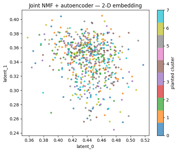
Even after only 10 epochs on CPU, the embedding shows structure that lines up with the planted clusters. With more epochs and real data, this becomes the input to downstream tasks — clustering, retrieval, classification.