Getting started
Alan Murphy, Brian Schilder, and Nathan Skene
Oct-22-2021
Source: vignettes/EWCE.Rmd
EWCE.RmdIntroduction
The EWCE R package is designed to facilitate expression weighted cell type enrichment analysis as described in our Frontiers in Neuroscience paper.1 EWCE can be applied to any gene list.
Using EWCE essentially involves two steps:
- Prepare a single-cell reference; i.e. CellTypeDataset (CTD). Alternatively, you can use one of the pre-generated CTDs we provide via the package
ewceData(which comes withEWCE).
- Run cell type enrichment on a gene list using the
bootstrap_enrichment_testfunction.
1. Prepare input data
CellTypeDataset
Load a CTD previously generated from mouse cortex and hypothalamus single-cell RNA-seq data (from the Karolinska Institute).
ctd <- ewceData::ctd()Plot CTD mean_exp
Plot the expression of four markers genes across all cell types in the CTD.
plt_exp <- EWCE::plot_ctd(ctd = ctd,
                          level = 1,
                          genes = c("Apoe","Gfap","Gapdh"),
                          metric = "mean_exp")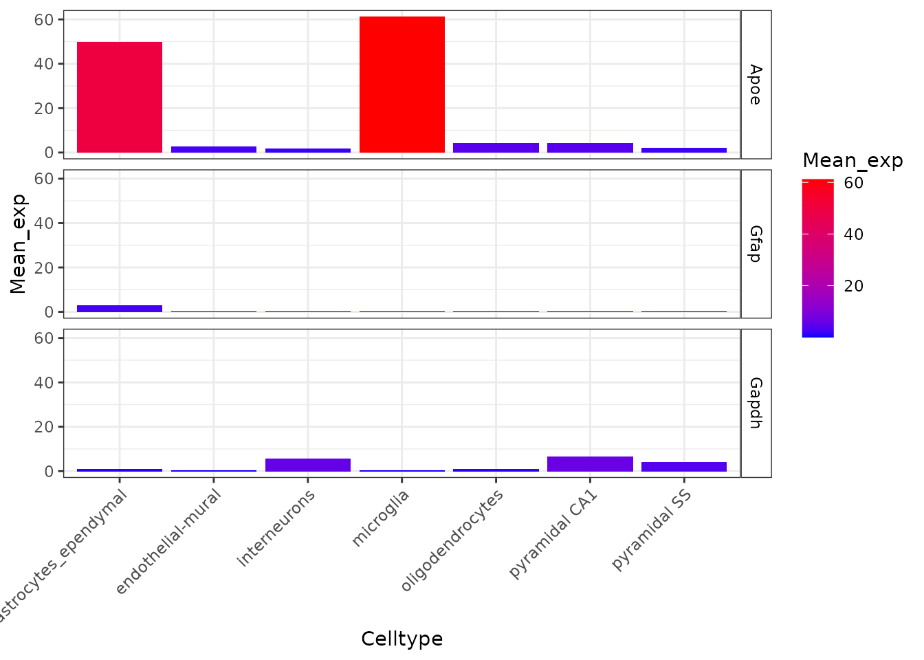
plt_spec <- EWCE::plot_ctd(ctd = ctd,
                           level = 2,
                           genes = c("Apoe","Gfap","Gapdh"),
                           metric = "specificity")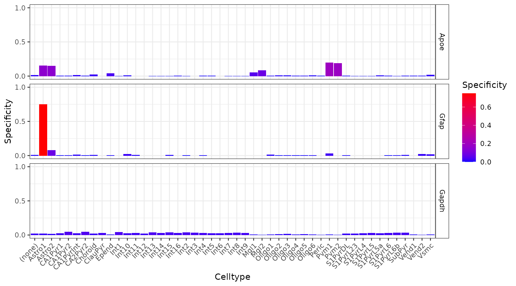
Gene list
Gene lists input into EWCE can comes from any source (e.g. GWAS, candidate genes, pathways).
Here, we provide an example gene list of Alzheimer’s disease-related nominated from a GWAS.
hits <- ewceData::example_genelist()
print(hits)
## [1] "APOE" "BIN1" "CLU" "ABCA7" "CR1" "PICALM"
## [7] "MS4A6A" "CD33" "MS4A4E" "CD2AP" "EOGA1" "INPP5D"
## [13] "MEF2C" "HLA-DRB5" "ZCWPW1" "NME8" "PTK2B" "CELF1"
## [19] "SORL1" "FERMT2" "SLC24A4" "CASS4"2. Run cell type enrichment tests
We now run the cell type enrichment tests on the gene list. Since the CTD is from mouse data (and is annotated using mouse genes) we specify the argument sctSpecies="mouse". bootstrap_enrichment_test will automaticlaly convert the mouse genes to human genes.
Since the gene list came from GWAS in humans, we set genelistSpecies="human".
Note: We set the seed at the top of this vignette to ensure reproducibility in the bootstrap sampling function.
Hyperparameters
Note: We use 100 repetitions here for the purposes of a quick example, but in practice you would want to use reps=10000 for publishable results.
reps <- 100
annotLevel <- 1
full_results <- EWCE::bootstrap_enrichment_test(sct_data = ctd,
                                                sctSpecies = "mouse",
                                                genelistSpecies = "human",
                                                hits = hits,
                                                reps = reps,
                                                annotLevel = annotLevel)
The main table of results is stored in full_results$results.
In this case, microglia were the only cell type that was significantly enriched in the Alzheimer’s disease gene list.
knitr::kable(full_results$results)| CellType | annotLevel | p | fold_change | sd_from_mean | q | |
|---|---|---|---|---|---|---|
| microglia | microglia | 1 | 0.00 | 2.0037539 | 3.8229690 | 0.000 |
| astrocytes_ependymal | astrocytes_ependymal | 1 | 0.11 | 1.3594176 | 1.4291523 | 0.385 |
| oligodendrocytes | oligodendrocytes | 1 | 0.78 | 0.7903958 | -0.8909301 | 1.000 |
| endothelial-mural | endothelial-mural | 1 | 0.83 | 0.7587306 | -0.9521828 | 1.000 |
| pyramidal SS | pyramidal SS | 1 | 0.84 | 0.8338200 | -0.9271986 | 1.000 |
| pyramidal CA1 | pyramidal CA1 | 1 | 0.90 | 0.7882024 | -1.1989117 | 1.000 |
| interneurons | interneurons | 1 | 1.00 | 0.3868205 | -3.1123590 | 1.000 |
The results can be visualised using another function, which shows for each cell type, the number of standard deviations from the mean the level of expression was found to be in the target gene list, relative to the bootstrapped mean.
The dendrogram at the top shows how the cell types are hierarchically clustered by transcriptional similarity.
plot_list <- EWCE::ewce_plot(total_res = full_results$results,
                             mtc_method = "BH",
                             ctd = ctd)
print(plot_list$withDendro)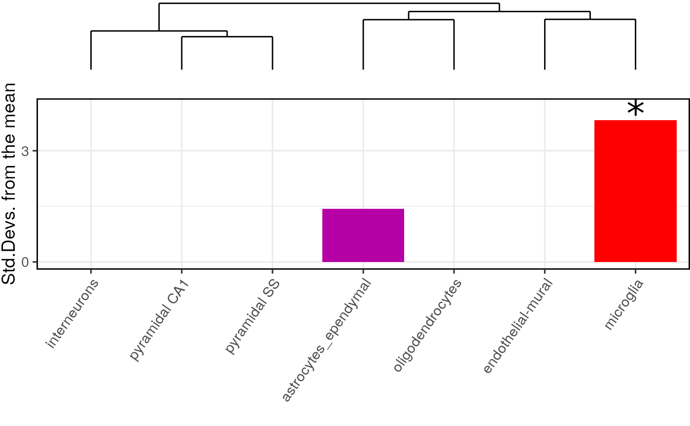
Session Info
utils::sessionInfo()## R version 4.1.1 (2021-08-10)
## Platform: x86_64-pc-linux-gnu (64-bit)
## Running under: Ubuntu 20.04.2 LTS
##
## Matrix products: default
## BLAS/LAPACK: /usr/lib/x86_64-linux-gnu/openblas-pthread/libopenblasp-r0.3.8.so
##
## locale:
## [1] LC_CTYPE=en_US.UTF-8 LC_NUMERIC=C
## [3] LC_TIME=en_US.UTF-8 LC_COLLATE=en_US.UTF-8
## [5] LC_MONETARY=en_US.UTF-8 LC_MESSAGES=C
## [7] LC_PAPER=en_US.UTF-8 LC_NAME=C
## [9] LC_ADDRESS=C LC_TELEPHONE=C
## [11] LC_MEASUREMENT=en_US.UTF-8 LC_IDENTIFICATION=C
##
## attached base packages:
## [1] stats graphics grDevices utils datasets methods base
##
## other attached packages:
## [1] ewceData_1.1.0 ExperimentHub_2.1.4 AnnotationHub_3.1.6
## [4] BiocFileCache_2.1.1 dbplyr_2.1.1 BiocGenerics_0.39.2
## [7] EWCE_2.0.0 RNOmni_1.0.0 BiocStyle_2.21.4
##
## loaded via a namespace (and not attached):
## [1] readxl_1.3.1 backports_1.2.1
## [3] systemfonts_1.0.3 plyr_1.8.6
## [5] lazyeval_0.2.2 orthogene_0.99.8
## [7] listenv_0.8.0 GenomeInfoDb_1.29.10
## [9] ggplot2_3.3.5 digest_0.6.28
## [11] htmltools_0.5.2 fansi_0.5.0
## [13] magrittr_2.0.1 memoise_2.0.0
## [15] openxlsx_4.2.4 limma_3.49.4
## [17] globals_0.14.0 Biostrings_2.61.2
## [19] matrixStats_0.61.0 pkgdown_1.6.1
## [21] colorspace_2.0-2 blob_1.2.2
## [23] rappdirs_0.3.3 textshaping_0.3.6
## [25] haven_2.4.3 xfun_0.27
## [27] dplyr_1.0.7 crayon_1.4.1
## [29] RCurl_1.98-1.5 jsonlite_1.7.2
## [31] glue_1.4.2 gtable_0.3.0
## [33] zlibbioc_1.39.0 XVector_0.33.0
## [35] HGNChelper_0.8.1 DelayedArray_0.19.4
## [37] car_3.0-11 future.apply_1.8.1
## [39] SingleCellExperiment_1.15.2 abind_1.4-5
## [41] scales_1.1.1 DBI_1.1.1
## [43] rstatix_0.7.0 Rcpp_1.0.7
## [45] viridisLite_0.4.0 xtable_1.8-4
## [47] foreign_0.8-81 bit_4.0.4
## [49] stats4_4.1.1 htmlwidgets_1.5.4
## [51] httr_1.4.2 ellipsis_0.3.2
## [53] farver_2.1.0 pkgconfig_2.0.3
## [55] sass_0.4.0 utf8_1.2.2
## [57] labeling_0.4.2 tidyselect_1.1.1
## [59] rlang_0.4.12 reshape2_1.4.4
## [61] later_1.3.0 AnnotationDbi_1.55.2
## [63] munsell_0.5.0 BiocVersion_3.14.0
## [65] cellranger_1.1.0 tools_4.1.1
## [67] cachem_1.0.6 generics_0.1.0
## [69] RSQLite_2.2.8 broom_0.7.9
## [71] evaluate_0.14 stringr_1.4.0
## [73] fastmap_1.1.0 yaml_2.2.1
## [75] ragg_1.1.3 babelgene_21.4
## [77] knitr_1.36 bit64_4.0.5
## [79] fs_1.5.0 zip_2.2.0
## [81] purrr_0.3.4 KEGGREST_1.33.0
## [83] gprofiler2_0.2.1 future_1.22.1
## [85] mime_0.12 compiler_4.1.1
## [87] plotly_4.10.0 filelock_1.0.2
## [89] curl_4.3.2 png_0.1-7
## [91] interactiveDisplayBase_1.31.2 ggsignif_0.6.3
## [93] tibble_3.1.5 bslib_0.3.1
## [95] homologene_1.4.68.19.3.27 stringi_1.7.5
## [97] highr_0.9 desc_1.4.0
## [99] forcats_0.5.1 lattice_0.20-45
## [101] Matrix_1.3-4 vctrs_0.3.8
## [103] pillar_1.6.4 lifecycle_1.0.1
## [105] BiocManager_1.30.16 jquerylib_0.1.4
## [107] cowplot_1.1.1 data.table_1.14.2
## [109] bitops_1.0-7 httpuv_1.6.3
## [111] patchwork_1.1.1 GenomicRanges_1.45.0
## [113] R6_2.5.1 bookdown_0.24
## [115] promises_1.2.0.1 gridExtra_2.3
## [117] rio_0.5.27 IRanges_2.27.2
## [119] parallelly_1.28.1 codetools_0.2-18
## [121] MASS_7.3-54 assertthat_0.2.1
## [123] SummarizedExperiment_1.23.5 rprojroot_2.0.2
## [125] withr_2.4.2 sctransform_0.3.2
## [127] S4Vectors_0.31.5 GenomeInfoDbData_1.2.7
## [129] parallel_4.1.1 hms_1.1.1
## [131] grid_4.1.1 tidyr_1.1.4
## [133] rmarkdown_2.11 MatrixGenerics_1.5.4
## [135] carData_3.0-4 ggpubr_0.4.0
## [137] Biobase_2.53.0 shiny_1.7.1