Applications to transcriptomes
Alan Murphy, Brian Schilder, and Nathan Skene
Oct-22-2021
Source: vignettes/transcriptomes.Rmd
transcriptomes.RmdApplication to transcriptomic data
Analysing single transcriptome study
For the prior analyses the gene lists were not associated with any numeric values or directionality. The methodology for extending this form of analysis to transcriptomic studies simply involves thresholding the most upregulated and downregulated genes.
To demonstrate this we have an example dataset tt_alzh. This data frame was generated using limma from a set of post-mortem tissue samples from Brodmann area 46 which were described in a paper by the Haroutunian lab1.
The first step is to load the data, obtain the MGI ids, sort the rows by t-statistic and then select the most up/down-regulated genes. The package then has a function ewce_expression_data which thresholds and selects the gene sets, and calls the EWCE function.
Below we show the function call using the default settings, but if desired different threshold values can be used, or alternative columns used to sort the table.
# ewce_expression_data calls bootstrap_enrichment_test so
tt_results <- EWCE:: ewce_expression_data(sct_data = ctd,
                                          tt = tt_alzh,
                                          annotLevel = 1,
                                          ttSpecies = "human",
                                          sctSpecies = "mouse")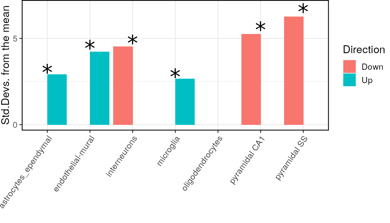
Generating bootstrap plots for transcriptomes
A common request is to explain which differentially expressed genes are associated with a cell type…
full_result_path <- EWCE::generate_bootstrap_plots_for_transcriptome(
  sct_data = ctd,
  tt = tt_alzh,
  annotLevel = 1,
  full_results = tt_results,
  listFileName = "examples",
  reps = reps,
  ttSpecies = "human",
  sctSpecies = "mouse",
  onlySignif = FALSE,
  savePath = tempdir())
Merging multiple transcriptome studies
Where multiple transcriptomic studies have been performed with the same purpose, i.e. seeking differential expression in dlPFC of post-mortem schizophrenics, it is common to want to determine whether they exhibit any shared signal. EWCE can be used to merge the results of multiple studies.
To demonstrate this we use a two further Alzheimer’s transcriptome datasets coming from Brodmann areas 36 and 44: these area stored in tt_alzh_BA36 and tt_alzh_BA44. The first step is to run EWCE on each of these individually and store the output into one list.
Load data
tt_alzh_BA36 <- ewceData::tt_alzh_BA36()
tt_alzh_BA44 <- ewceData::tt_alzh_BA44()
Run EWCE analysis
tt_results_36 <- EWCE::ewce_expression_data(sct_data = ctd,
                                             tt = tt_alzh_BA36,
                                             annotLevel = 1,
                                             ttSpecies = "human",
                                             sctSpecies = "mouse")
tt_results_44 <- EWCE::ewce_expression_data(sct_data = ctd,
                                             tt = tt_alzh_BA44,
                                             annotLevel = 1,
                                             ttSpecies = "human",
                                             sctSpecies = "mouse")

# Fill a list with the results
results <- EWCE::add_res_to_merging_list(tt_results)
results <- EWCE::add_res_to_merging_list(tt_results_36,results)
results <- EWCE::add_res_to_merging_list(tt_results_44,results)

# Perform the merged analysis
# For publication reps should be higher
merged_res <- EWCE::merged_ewce(results = results,
                                reps = 10)
print(merged_res)
The results can then be plotted as normal using the ewce_plot function.
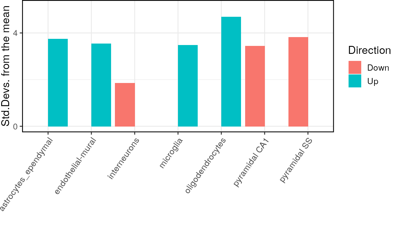
The merged results from all three Alzheimer’s brain regions are found to be remarkably similar, as was reported in our paper.
Session Info
utils::sessionInfo()## R version 4.1.1 (2021-08-10)
## Platform: x86_64-pc-linux-gnu (64-bit)
## Running under: Ubuntu 20.04.2 LTS
##
## Matrix products: default
## BLAS/LAPACK: /usr/lib/x86_64-linux-gnu/openblas-pthread/libopenblasp-r0.3.8.so
##
## locale:
## [1] LC_CTYPE=en_US.UTF-8 LC_NUMERIC=C
## [3] LC_TIME=en_US.UTF-8 LC_COLLATE=en_US.UTF-8
## [5] LC_MONETARY=en_US.UTF-8 LC_MESSAGES=C
## [7] LC_PAPER=en_US.UTF-8 LC_NAME=C
## [9] LC_ADDRESS=C LC_TELEPHONE=C
## [11] LC_MEASUREMENT=en_US.UTF-8 LC_IDENTIFICATION=C
##
## attached base packages:
## [1] stats graphics grDevices utils datasets methods base
##
## other attached packages:
## [1] ewceData_1.1.0 ExperimentHub_2.1.4 AnnotationHub_3.1.6
## [4] BiocFileCache_2.1.1 dbplyr_2.1.1 BiocGenerics_0.39.2
## [7] EWCE_2.0.0 RNOmni_1.0.0 BiocStyle_2.21.4
##
## loaded via a namespace (and not attached):
## [1] readxl_1.3.1 backports_1.2.1
## [3] systemfonts_1.0.3 plyr_1.8.6
## [5] lazyeval_0.2.2 orthogene_0.99.8
## [7] listenv_0.8.0 GenomeInfoDb_1.29.10
## [9] ggplot2_3.3.5 digest_0.6.28
## [11] htmltools_0.5.2 fansi_0.5.0
## [13] magrittr_2.0.1 memoise_2.0.0
## [15] openxlsx_4.2.4 limma_3.49.4
## [17] globals_0.14.0 Biostrings_2.61.2
## [19] matrixStats_0.61.0 pkgdown_1.6.1
## [21] colorspace_2.0-2 blob_1.2.2
## [23] rappdirs_0.3.3 textshaping_0.3.6
## [25] haven_2.4.3 xfun_0.27
## [27] dplyr_1.0.7 crayon_1.4.1
## [29] RCurl_1.98-1.5 jsonlite_1.7.2
## [31] glue_1.4.2 gtable_0.3.0
## [33] zlibbioc_1.39.0 XVector_0.33.0
## [35] HGNChelper_0.8.1 DelayedArray_0.19.4
## [37] car_3.0-11 future.apply_1.8.1
## [39] SingleCellExperiment_1.15.2 abind_1.4-5
## [41] scales_1.1.1 DBI_1.1.1
## [43] rstatix_0.7.0 Rcpp_1.0.7
## [45] viridisLite_0.4.0 xtable_1.8-4
## [47] foreign_0.8-81 bit_4.0.4
## [49] stats4_4.1.1 htmlwidgets_1.5.4
## [51] httr_1.4.2 ellipsis_0.3.2
## [53] farver_2.1.0 pkgconfig_2.0.3
## [55] sass_0.4.0 utf8_1.2.2
## [57] tidyselect_1.1.1 rlang_0.4.12
## [59] reshape2_1.4.4 later_1.3.0
## [61] AnnotationDbi_1.55.2 munsell_0.5.0
## [63] BiocVersion_3.14.0 cellranger_1.1.0
## [65] tools_4.1.1 cachem_1.0.6
## [67] generics_0.1.0 RSQLite_2.2.8
## [69] broom_0.7.9 evaluate_0.14
## [71] stringr_1.4.0 fastmap_1.1.0
## [73] yaml_2.2.1 ragg_1.1.3
## [75] babelgene_21.4 knitr_1.36
## [77] bit64_4.0.5 fs_1.5.0
## [79] zip_2.2.0 purrr_0.3.4
## [81] KEGGREST_1.33.0 gprofiler2_0.2.1
## [83] future_1.22.1 mime_0.12
## [85] compiler_4.1.1 plotly_4.10.0
## [87] filelock_1.0.2 curl_4.3.2
## [89] png_0.1-7 interactiveDisplayBase_1.31.2
## [91] ggsignif_0.6.3 tibble_3.1.5
## [93] bslib_0.3.1 homologene_1.4.68.19.3.27
## [95] stringi_1.7.5 highr_0.9
## [97] desc_1.4.0 forcats_0.5.1
## [99] lattice_0.20-45 Matrix_1.3-4
## [101] vctrs_0.3.8 pillar_1.6.4
## [103] lifecycle_1.0.1 BiocManager_1.30.16
## [105] jquerylib_0.1.4 cowplot_1.1.1
## [107] data.table_1.14.2 bitops_1.0-7
## [109] httpuv_1.6.3 patchwork_1.1.1
## [111] GenomicRanges_1.45.0 R6_2.5.1
## [113] bookdown_0.24 promises_1.2.0.1
## [115] gridExtra_2.3 rio_0.5.27
## [117] IRanges_2.27.2 parallelly_1.28.1
## [119] codetools_0.2-18 MASS_7.3-54
## [121] assertthat_0.2.1 SummarizedExperiment_1.23.5
## [123] rprojroot_2.0.2 withr_2.4.2
## [125] sctransform_0.3.2 S4Vectors_0.31.5
## [127] GenomeInfoDbData_1.2.7 parallel_4.1.1
## [129] hms_1.1.1 grid_4.1.1
## [131] tidyr_1.1.4 rmarkdown_2.11
## [133] MatrixGenerics_1.5.4 carData_3.0-4
## [135] ggpubr_0.4.0 Biobase_2.53.0
## [137] shiny_1.7.1